Research
Broadly, my research interests involve computational biology and general mathematical modelling of biological processes, systems, and phenomena. In particular, I am currently interested in applying machine learning/artificial intelligence techniques in tandem with differential equations and stochastic models to answer questions of cancer stem cell evolution and treatment response in the study of human cancers. I find biological systems to be fascinating in their complexity and hope to elucidate their behaviour by using stochastic machine learning techniques coupled with traditional models. After all, nature has no compunction to regulate towards easy description even if it does so in aggregate.
Theses
-

Machine Learning Techniques and Stochastic Modeling in Mathematical Oncology Ph.D. Thesis Jul 18, 2022
Brydon Eastman
-

Sensitivity to predator response functions in the chemostat Master's Thesis Aug 7, 2017
Brydon Eastman
There are a variety of types of mathematical models called predator-prey models. In these models there is one being (whether an animal, or a bacteria population, or some other example) called the predator that consumes the prey. There is implicitly some benefit to this for the predator which mathematically we represent by the predator response function.
Roughly, the predator respponse function represents the fitness benefit to the predator for consuming a certain amount of prey. Typically the predator response function is a saturating function such that it's always positive, always increasing, and always less than some total capacity. The intuition is like this: initially it's good for the predator to eat prey, since the alternative is starvation of the predator. However, past a certain point the
Biological models of predator-prey interaction have been shown to have high sensitivity to the functional form of the predator response (see [3]). Chemostat models with competition have been shown to be robust under various forms of response function (see [15]). The focus here is restricted to a simple chemostat model with predator-prey dynamics. Several functional responses of Holling Type II form are considered. The sensitivity of dynamics to our choice of functional form is demonstrated by way of bifurcation theory. These results should be a warning to modelers, since by data collection and curve-fitting alone it is impossible to determine the exact functional form of the predator response function.
Publications
You can view these publications by clicking the images of the papers. Most of these are open-access, but if you have any issues accessing the PDFs for any reason contact me and I would be more than happy to assist. For each of these publications I include a summary that can be viewed. These summaries are written with the intention that an undergraduate student could gain a birds-eye-view of the content of the research article.
-

A PINN Approach to Symbolic Differential Operator Discovery with Sparse Data NeurIPS 2022 and ICML 2023 Dec 9, 2022
Lena Podina, Brydon Eastman, Mohammad Kohandel
Some placeholder content for the collapse component. This panel is hidden by default but revealed when the user activates the relevant trigger.
Given ample experimental data from a system governed by differential equations, it is possible to use deep learning techniques to construct the underlying differential operators. In this work we perform symbolic discovery of differential operators in a situation where there is sparse experimental data. This small data regime in machine learning can be made tractable by providing our algorithms with prior information about the underlying dynamics. Physics Informed Neural Networks (PINNs) have been very successful in this regime (reconstructing entire ODE solutions using only a single point or entire PDE solutions with very few measurements of the initial condition). We modify the PINN approach by adding a neural network that learns a representation of unknown hidden terms in the differential equation. The algorithm yields both a surrogate solution to the differential equation and a black-box representation of the hidden terms. These hidden term neural networks can then be converted into symbolic equations using symbolic regression techniques like AI Feynman. In order to achieve convergence of these neural networks, we provide our algorithms with (noisy) measurements of both the initial condition as well as (synthetic) experimental data obtained at later times. We demonstrate strong performance of this approach even when provided with very few measurements of noisy data in both the ODE and PDE regime. -

A comparison and calibration of integer and fractional order models of COVID-19 with stratified public response Mathematical Biosciences and Engineering Sept 1, 2022
Somayeh Fouladi, Mohammad Kohandel, Brydon Eastman
Some placeholder content for the collapse component. This panel is hidden by default but revealed when the user activates the relevant trigger.
The spread of SARS-CoV-2 in the Canadian province of Ontario has resulted in millions of infections and tens of thousands of deaths to date. Correspondingly, the implementation of modeling to inform public health policies has proven to be exceptionally important. In this work, we expand a previous model of the spread of SARS-CoV-2 in Ontario, "Modeling the impact of a public response on the COVID-19 pandemic in Ontario," to include the discretized, Caputo fractional derivative in the susceptible compartment. We perform identifiability and sensitivity analysis on both the integer-order and fractional-order SEIRD model and contrast the quality of the fits. We note that both methods produce fits of similar qualitative strength, though the inclusion of the fractional derivative operator quantitatively improves the fits by almost 27% corroborating the appropriateness of fractional operators for the purposes of phenomenological disease forecasting. In contrasting the fit procedures, we note potential simplifications for future study. Finally, we use all four models to provide an estimate of the time-dependent basic reproduction number for the spread of SARS-CoV-2 in Ontario between January 2020 and February 2021. -

Reinforcement learning derived chemotherapeutic schedules for robust patient-specific therapy Nature Scientific Reports Sep 9, 2021
Brydon Eastman, Michelle Pzedborski, Mohammad Kohandel
View summary or view the asbstract.
This project was presented as a poster at the 2021 meeting of the Society for Mathematical Biology for which I received the Applied BioMath Poster Prize. Here are the links to the video of the poster presentation and to the poster itself.
The in-silico development of a chemotherapeutic dosing schedule for treating cancer relies upon a parameterization of a particular tumour growth model to describe the dynamics of the cancer in response to the dose of the drug. In practice, it is often prohibitively difficult to ensure the validity of patient-specific parameterizations of these models for any particular patient. As a result, sensitivities to these particular parameters can result in therapeutic dosing schedules that are optimal in principle not performing well on particular patients. In this study, we demonstrate that chemotherapeutic dosing strategies learned via reinforcement learning methods are more robust to perturbations in patient-specific parameter values than those learned via classical optimal control methods. By training a reinforcement learning agent on mean-value parameters and allowing the agent periodic access to a more easily measurable metric, relative bone marrow density, for the purpose of optimizing dose schedule while reducing drug toxicity, we are able to develop drug dosing schedules that outperform schedules learned via classical optimal control methods, even when such methods are allowed to leverage the same bone marrow measurements. -

Modeling the impact of public response on the COVID-19 pandemic in Ontario PLoS One Apr 14, 2021
Brydon Eastman, Cameron Meaney, Michelle Pzedborski, Mohammad Kohandel
Some placeholder content for the collapse component. This panel is hidden by default but revealed when the user activates the relevant trigger.The outbreak of SARS-CoV-2 is thought to have originated in Wuhan, China in late 2019 and has since spread quickly around the world. To date, the virus has infected tens of millions of people worldwide, compelling governments to implement strict policies to counteract community spread. Federal, provincial, and municipal governments have employed various public health policies, including social distancing, mandatory mask wearing, and the closure of schools and businesses. However, the implementation of these policies can be difficult and costly, making it imperative that both policy makers and the citizenry understand their potential benefits and the risks of non-compliance. In this work, a mathematical model is developed to study the impact of social behaviour on the course of the pandemic in the province of Ontario. The approach is based upon a standard SEIRD model with a variable transmission rate that depends on the behaviour of the population. The model parameters, which characterize the disease dynamics, are estimated from Ontario COVID-19 epidemiological data using machine learning techniques. A key result of the model, following from the variable transmission rate, is the prediction of the occurrence of a second wave using the most current infection data and disease-specific traits. The qualitative behaviour of different future transmission-reduction strategies is examined, and the time-varying reproduction number is analyzed using existing epidemiological data and future projections. Importantly, the effective reproduction number, and thus the course of the pandemic, is found to be sensitive to the adherence to public health policies, illustrating the need for vigilance as the economy continues to reopen. -

A Predator-Prey Model in the Chemostat with Holling Type II Response Function Mathematics in Applied Sciences and Engineering Nov 1, 2020
Tedra Bolger, Brydon Eastman, Madeleine Hill, Gail S. K. Wolkowicz
Some placeholder content for the collapse component. This panel is hidden by default but revealed when the user activates the relevant trigger.A model of predator-prey interaction in a chemostat with Holling Type II predator functional response of the Monod or Michaelis-Menten form, is considered. It is proved that local asymptotic stability of the coexistence equilibrium implies that it is globally asymptotically stable. It is also shown that when the coexistence equilibrium exists, but is unstable, solutions converge to a unique, orbitally asymptotically stable periodic orbit. Thus the range of the dynamics of the chemostat predator-prey model is the same as for the analogous classical Rosenzweig-MacArthur predator-prey model with Holling Type II functional response. An extension that applies to other functional responses is also given. -

The effects of phenotypic plasticity on the fixation probability of mutant cancer stem cells Journal of Theoretical Biology Oct 21, 2020
Brydon Eastman, Dominik Wodarz, Mohammad Kohandel
Some placeholder content for the collapse component. This panel is hidden by default but revealed when the user activates the relevant trigger.The cancer stem cell hypothesis claims that tumor growth and progression are driven by a (typically) small niche of the total cancer cell population called cancer stem cells (CSCs). These CSCs can go through symmetric or asymmetric divisions to differentiate into specialised, progenitor cells or reproduce new CSCs. While it was once held that this differentiation pathway was unidirectional, recent research has demonstrated that differentiated cells are more plastic than initially considered. In particular, differentiated cells can de-differentiate and recover their stem-like capacity. Two recent papers have considered how this rate of plasticity affects the evolutionary dynamic of an invasive, malignant population of stem cells and differentiated cells into existing tissue (Mahdipour-Shirayeh et al., 2017; Wodarz, 2018). These papers arrive at seemingly opposing conclusions, one claiming that increased plasticity results in increased invasive potential, and the other that increased plasticity decreases invasive potential. Here, we show that what is most important, when determining the effect on invasive potential, is how one distributes this increased plasticity between the compartments of resident and mutant-type cells. We also demonstrate how these results vary, producing non-monotone fixation probability curves, as inter-compartmental plasticity changes when differentiated cell compartments are allowed to continue proliferating, highlighting a fundamental difference between the two models. We conclude by demonstrating the stability of these qualitative results over various parameter ranges. Keywords: cancer stem cells, plasticity, de-differentiation, fixation probability. -

From Solid-State NMR to Crystal Structures through Combinatorial Tiling Theory Int. Union Crystallography Jan 1, 2018
Darren Brouwer, Janelle Vanderhout, Chelsey Hurst, Brydon Eastman
Some placeholder content for the collapse component. This panel is hidden by default but revealed when the user activates the relevant trigger.Solid-state NMR spectroscopy can provide a great deal of structural information about the local environments of NMR-active nuclei. When combined with other complementary techniques such as diffraction and quantum chemical calculations – an approach referred to as NMR crystallography – powerful structure determination strategies emerge that allow for the elucidation of detailed structures that no one technique could provide on its own. We have been particularly interested in developing structure solution strategies that maximally exploit the structural information available in 1D and 2D solid state NMR data from network materials such as zeolites, with a view to being able to solve structures when minimal diffraction data is available, such as disordered layered structures. Based on some elegant mathematics in the area of combinatorial tiling theory, we are developing a novel structure solution strategy for network materials that will efficiently generate all feasible structures that arise from the number of sites (number of peaks), relative site occupancies (peak intensities), coordination environments (chemical shifts) revealed in 1D solid-state NMR spectra and the inter-site connectivities (cross peak intensities) revealed in 2D correlation spectra. One of the key features of this approach is that no prior knowledge of the crystallographic space group or unit cell parameters is intrinsically necessary, which in principle allows for the generation of network crystal structures directly from solid-state NMR data alone. This talk will introduce and explain Delaney symbols (mathematical structures for describing tilings of the 2D plane or 3D space), highlighting the rich amount of structural information that they contain and how they allow for novel conceptual linkages between solid-state NMR and crystallography of network materials. -

Pentadiagonal Companion Matrices Special Matrices Oct 28, 2015
Brydon Eastman and Kevin N. Vander Meulen
View summary or view the abstract.
There's a lot in this paper I'm proud of. This paper was the "capstone project" for my honours mathematics major in undergraduate. Below I talk about how we classified all sparse companion matrices (and you should probably read that summary before this one, as I reference a lot of the ideas there). I also talked about how there are different representations of the same matrix that are isomorphic in a certain sense under transpose and permutation similarity (or relabelling vertices of the associated digraph). Now linear algebra underlies a surprising amount of computational mathematics (from solutions of PDEs to neural networks to Fourier transforms) and there are certain algorithms that work really well with matrices of certain "band-width". Thinking in diagonals, there are the so-called tri-diagonal matrices, matrices where everything is zero except the main diagonal and the first super and sub diagonal. We show that no tri-diagonal matrix can be a companion matrix. Next up are the penta-diagonal matrices (you have the main diagonal, the first two super-diagonals, and the first two sub-diagonals). Now we already knew that some companion matrices could be represented in a pentadiagonal form, so our next question was: which ones? In this paper we classified all the sparse pentadiagonal companion matrices.
How did we do this? Well, graph theory was our trusty tool so we first applied graph theory. In so doing we were able to isolate which of our companion matrices would be pentadiagonal. They corresponded to those graphs that were subgraphs of a "strut".
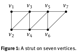
We then algebraically express all of these matrices in pentadiagonal form and in so doing we discover that all the pentadiagonal companion matrices happen to belong to Fiedler's class.
But remember how in that original companion matrix paper we didn't really care about the labelling of these vertices? There's a sense that relabelling the vertices gives you the "same" graph. And it does, that is true. But we're not interested in graphs right now, right now we're interested in matrices. And relabelling these vertices can take a matrix that has a pentadiagonal form (under some particular labelling) and place it in a form that isn't pentadiagonal. (In fact, in that original matrix way of presenting companion matrices that I discuss below, for large enough \(n\) none of those matrices are pentadiagonal as presented, even if they're equivalent to a pentadiagonal matrix).
So our next question was: great, now that we've identified all the sparse companion matrices that possess a pentadiagonal form, how do we recover the permutation that takes them from the "standard form" into this pentadiagonal form? This makes up the bulk of the back-half of the paper. This is where I had a moment where I felt very, very clever. Remember how we can express Fiedler's matrices in standard form as a lattice path, well this lattice path has many "corners". We recognized that if we counted how many steps you took before you turned a corner, you'd have this "flight length sequence", and I found a way to go from this flight-length sequence to the permutation required.
A much cleaner version of the method I uncovered is in the paper. The original method was very, very strange. I remember sitting in my undergraduate thesis advisors office explaining the process to him ("you start with the biggest number that's in the middle, then you slide the numbers until you hit a number bigger than yourself, you can't cross that, but you're trying to get everything as ascending as possible without crossing numbers bigger than yourself, except...") and after 30 minutes of me presenting my scatter-brained algorithm and Maple code that corroborated my idea he paused, sighed, and said "yes I see that this seems true, how on Earth can you ever prove that?". I had worked with him on many projects at this point and he had carefully steered me away from many impossible proofs that I had attempted in the past, so I recognised the message underneath his words. It was the same voice he used when talking to me about Collatz' conjecture or about my hail-mary attempt at proving the \(2n\) conjecture for zero-nonzero patterns the year prior. I can't remember how many meetings we had after that, but I do remember when I presented to him the water-tight proof (complete with so, so much mathematical machinery). We whittled away at that proof (though fundamentally, it is the same argument) to present the version we have in the paper (while it's slightly less scatter-brained with slightly less machinery, it is still a bit scatter-brained and does contain an inordinate amount of definitions).
There aren't many moments in life where you get to do the impossible, and very little in life is guaranteed, but I've always revered mathematics as a field that effectively guarantees the provision of plenty of opportunities to whittle away at weird, weird problems until the stars align and a result falls out. Once I worked with an analytical chemistry postdoc who said to me, in a slightly condescending tone, "isn't linear algebra done?" Oh boy, if only he knew. The soaring towers have been climbed, sure, but there's still plenty of monsters left in the basement.
The class of sparse companion matrices was recently characterized in terms of unit Hessenberg matrices. We determine which sparse companion matrices have the lowest bandwidth, that is, we characterize which sparse companion matrices are permutationally similar to a pentadiagonal matrix and describe howto find the permutation involved. In the process, we determine which of the Fiedler companion matrices are permutationally similar to a pentadiagonal matrix. We also describe how to find a Fiedler factorization, up to transpose, given only its corner entries. -

Sparse Spectrally Arbitrary Patterns The Electronic Journal of Linear Algebra Apr 28, 2015
Brydon Eastman, Bryan Shader, Kevin N. Vander Meulen
View summary or view the abstract.
The word "matrix" shares the same root-words as "maternal" for a reason. Matrices were originally named because of their capacity to "give birth" to "eigenvalues". Once you've realised this you'll see just how heavy-handed some of the symbolism in the film was.

So eigenvalues - literally "special values" - are so important that we named the whole mathematical object in an oblique way after them. For a while now people have been studying how the arrangement of both zero and non-zero entries in a matrix restricts what possible eigenvalues that matrix can permit. This has applications for a variety of reasons - in biology for instance, next-generation matrices are useful and the value of the largest eigenvalue plays a role in predicting the long-term dynamics of these Markovian systems. We also a-priori often know the placement of zero and non-zero entries in such a matrix, even if we don't know the particular value of the non-zero entries.
In particular for these patterns people are interested in which patterns are spectrally arbitrary. This is just a fancy way of saying that these matrix patterns can produce any set of eigenvalues you want.
\(\require{ams}\)In this paper we considered spectrally arbitrary patterns of a slightly different type. We stratify the elements of our matrix pattern into two classes: entries that are definitely zero, definitely non-zero, and entries that are variable (either zero or nonzero). Now we were interested in the sparse patterns. In this sense, sparse just means "having a lot of zeros". At this point it was well known that in an \(n\times n\) pattern, you couldn't have more than \((n-1)^2\) zeros and still have the pattern be spectrally arbitrary. In other words, you need at least \(2n-1\) potentially non-zero entries in order to have a spectrally arbitrary pattern. In an arduous fashion we completely classify all the \(2\times 2\) and \(3\times 3\) spectrally arbitrary patterns. Along the way, we discovered something neat. We found a large class of sparse matrix patterns that are spectrally arbitrary for any \(n\). (As an aside: it was in working on this result that we established the companion matrix result below). As in the companion matrix paper, you start with an \(n\times n\) matrix with non-zero entries on the super-diagonal (represented by \(\ast\)) and then place remaining \(n\) variable entries on each sub-diagonal (represented by (\(\circledast\)). It doesn't matter where you place those entries on their respective diagonals, just so long as you put one on each of the \(n\) diagonals.
How did we prove this? Well, there's this kind-of-technical tool called the Nilpotent-Jacobian method that we used. This worked for this class and we were able to demonstrate that these sparse patterns were spectrally arbitrary for any \(n\). I remember falling asleep some weeks with visions of circle-asterisks slipping and sliding along diagonals like penguins. So this NJ method seemed pretty powerful! It's one of those methods that when it works, it works; but when it fails, you learn nothing. That is to say, if the NJ method gives you a non-zero result at the end, you know your pattern is spectrally arbitrary, but if it gives you a zero result you learn absolutely nothing. It might not be spectrally arbitrary or it might be; you're on your own.
While working with this diagonal-slide pattern (we ended up calling it the super-pattern of the companion matrices), we found a similar class of sparse spectrally arbitary patterns where you can "double up" variable entries along certain diagonals by removing an entry from a different diagonal. The NJ method failed on these patterns leaving us with no information. We were able to demonstrate the spectrally arbitrary property of these class of patterns directly, however, by demonstrating that one could achieve any characteristic polynomial they wanted with the pattern.
We explore combinatorial matrix patterns of order n for which some matrix entries are necessarily nonzero, some entries are zero, and some are arbitrary. In particular, we are interested in when the pattern allows any monic characteristic polynomial with real coefficients, that is, when the pattern is spectrally arbitrary. We describe some order n patterns that are spectrally arbitrary. We show that each superpattern of a sparse companion matrix pattern is spectrally arbitrary. We determine all the minimal spectrally arbitrary patterns of order 2 and 3. Finally, we demonstrate that there exist spectrally arbitrary patterns for which the nilpotent-Jacobian method fails. -

Companion Matrix Patterns Linear Algebra and its Applications Feb 1, 2014
Brydon Eastman, I.-J. Kim, B.L. Shader, K.N. Vander Meulen
View summary or view the abstract.
This is a very fun paper. It started out as trying to solve a related linear algebra problem, then evolved into an exploration of the related (di)graph theory. Finally we ended up proving something fundamental about a building block of mathematics. I was once asked "what of your work will be impactful in 100 years". I'm not sure if I know the full answer to that question, but I think this result will be among them. I believe this result belays fundamental information about building blocks of some of the most important mathematical objects. I'm quite honoured to have been a part of this work and am proud of my contributions to it.
A companion matrix is simply a matrix where one inserts variable entries \(-a_1\), \(-a_2\), \(\ldots\), \(-a_n\) and the resulting matrix has the characteristic polynomial with these entries as coefficients, that is the characteristic polynomial is \(x^n+a_1\,x^{n-1}+\cdots+a_n\). The most famous of these is the so-called Frobenius companion matrix (first suggested by Frobenius in 1878). Turns out, there are many applications of this matrix and matrices of this kind in fields ranging from numeric solutions of polynomials to optimal control theory. This shouldn't be terribly surprising, polynomials are an incredibly important class of elementary function and matrices underlie a surprising majority of computational mathematics. In fact, matrices are named after their capacity to encode the roots of polynomials in eigenvalues, but that's a much larger story. Back to companion matrices: as an example, the degree 4 Frobenius companion matrix can be represented as \[ \left[ \begin{array}{cccc} -a_1&1&0&0\\ -a_2&0&1&0\\ -a_3&0&0&1\\ -a_4&0&0&0\\ \end{array} \right]. \]
The above matrix is very simple (in the sense that it's just my variable entries, 1s, and 0s). In fact, most of the matrix is composed of 0s. Such matrices are called sparse. It is well known that this is as sparse as you can get -- meaning, for an \(n\times n\) matrix to be able to encode any characteristic polynomial, you need at least \(2n-1\) entries in the matrix. In Frobenius' companion matrix we get this from the \(n\) variable entries and the \(n-1\) unit entries on the super-diagonal. In 2003, Fiedler greatly expanded this class of sparse companion matrices. Two such examples are given below (though there are more! In fact, there are \(2^{n-2}\) "unique" Fiedler companion matrices of order \(n\) (I'm being a bit coy about my use of the word "unique" there, it's technical, we explain more in the paper!)).
\( \left[ \begin{array}{cccc} 0&1&0&0\\ 0&-a_1&1&0\\ -a_3&-a_2&0&1\\ -a_4&0&0&0\\ \end{array} \right]\) \( \left[ \begin{array}{cccc} 0&1&0&0\\ 0&0&1&0\\ -a_3&-a_2&-a_1&1\\ -a_4&0&0&0\\ \end{array} \right] \)
We were actually trying to solve a completely different problem on spectrally arbitrary patterns (discussed in a paper above) when we stumbled across a new class of companion matrices. I still remember the day that I was able to demonstrate that this new class would always result in a companion matrix and provided an argument that was geometric both in the matrix expression and in the underlying graph theoretic expression. Working that result out on the whiteboard is one of those memories that I think I will carry with me throughout my life. My co-authors were able to demonstrate the (suprising and very exciting) reverse direction, but I'm getting ahead of myself. What even is this class of matrices and how do I build one? It's not terribly difficult, but you'll have to tilt your head a little and think in terms of diagonals.
I already mentioned that the Frobenius companion matrix has only 1s on its super-diagonal. What I mean by this is, if you tilt your head slightly, you'll notice all the 1s lie in a straight diagonal line. If we think of these matrices as stacks of diagonal lines (instead of rows of horizontal ones), we can see that Frobenius' companion matrix has two zero diagonals, one diagonal of all 1s, one diagonal with only \(-a_1\) (and the rest zeros), another diagonal with only \(-a_2\) (and the rest zeros), et cetera until we reach the final diagonal with only \(-a_n\). Now look at one of Fiedler's companion matrix -- it follows the same pattern! Only 0s, only 0s, only 1s, only 0s and a single \(-a_1\) term, etc. We can show that all of Fiedler's companion matrices follow this approach. In fact, we can demonstrate that we can build any of Fiedler's companion matrices by following the simple strategy: start with a matrix like this \[\left[ \begin{array}{cccc} 0&1&0&0\\ 0&0&1&0\\ 0&0&0&1\\ -a_4&0&0&0\\ \end{array} \right]\] and, finally, fill in the rest of the entries in a "lattice-path". This just means, place your \(-a_3\) entry so that it's either above or beside your \(-a_4\) entry, next place your \(-a_2\) so that it's either above or beside the \(-a_3\) entry, etc. I like to think of it like laying tiles in a garden.
\(\left[ \begin{array}{cccc} 0&1&0&0\\ 0&0&1&0\\ 0&-a_2&-a_1&1\\ -a_4&-a_3&0&0\\ \end{array} \right]\) \( \left[ \begin{array}{cccc} 0&1&0&0\\ 0&0&1&0\\ 0&0&-a_1&1\\ -a_4&-a_3&-a_2&0\\ \end{array} \right]\) \( \left[ \begin{array}{cccc} 0&1&0&0\\ 0&0&1&0\\ -a_3&-a_2&-a_1&1\\ -a_4&0&0&0\\ \end{array} \right]\) \( \left[ \begin{array}{cccc} 0&1&0&0\\ 0&-a_1&1&0\\ -a_3&-a_2&0&1\\ -a_4&0&0&0\\ \end{array} \right]\)
This process introduces a lot of choice! That's why Fiedler has many companion matrices and not just the one. Also note that for larger order (like a \(5\times 5\) or \(10\times 10\) matrix) you can get even more choices. There's some fuzzy details about which of these choices end up with a "unique" result, turns out your first choice is "fixed" (up to a permutation-transpose isomorphism), which is why I said that Fiedler's process matrices are a class of size \(2^{n-2}\) not \(2^{n-1}\). (The two comes because you're always choosing either above or beside, we'd expect the answer to be \(2^{n-1}\) as we're placing \(n-1\) entries (the \(-a_n\) entry is always in the bottom-left corner)). Also note that if we chose "up" for every choice we'd recover Frobenius' original companion matrix! So Fiedler's class expands the way we think about companion matrices.
(At this point I'd like to point out that this is not how Fiedler originally thought of, or counted, his companion matrices. He presented a beautiful construction by multiplying elementary matrices in his original paper that is definitely worth visiting. This geometric approach is just a useful thing we uncovered in our investigation that I find very compelling. It also has a very nice graph theory analogue!)
While this is a cool new way of viewing Fiedler's matrices, how does this relate back to our new result? Well, the process is similar: you start with the basic \[\left[ \begin{array}{cccc} 0&1&0&0\\ 0&0&1&0\\ 0&0&0&1\\ -a_4&0&0&0\\ \end{array} \right]\] matrix except your next step is to place the \(-a_1\), main-diagonal entry (anywhere is fine!). \[\left[ \begin{array}{cccc} 0&1&0&0\\ 0&0&1&0\\ 0&0&-a_1&1\\ -a_4&0&0&0\\ \end{array} \right]\] Now we have to place the remaining \(n-2\) entries. You place these anywhere on their respective diagonals as long as they fall within the imaginary box with the \(-a_n\) entry in the bottom-left corner and the \(-a_1\) entry in the top-right corner \[\left[ \begin{array}{cccc} 0&1&0&0\\ 0&0&1&0\\ -a_3&0&-a_1&1\\ -a_4&0&-a_2&0\\ \end{array} \right].\]
You'll see that this includes not only Frobenius' companion matrix (just place the \(-a_1\) in the top-left of the matrix and every other choice is forced) but also every one of Fiedler's companion matrices. Moreover you get matrices (like the one above) that are companion matrices that do not belong in Fiedler's class (note that the lattice-path is broken!).
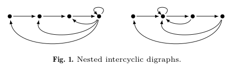
Why does this work? Well, that gets a bit too complicated to explain in a web-format like this, but you can write any matrix as a directed-graph. The 1s on the super-diagonal then form a directed Hamilton path across our \(n\) vertices and the variable entries \(-a_k\) point backwards creating \(k\)-cycles along this Hamilton path. It turns out, if all these \(k\) cycles are nested within each other, you get a Fiedler companion matrix. If all these \(k\) cycles share at least one common vertex, you get one of our larger class of companion matrices. We call these types of graphs nested-intercyclic and intercyclic respectively. (By having the \(k\)-cycles all share a vertex we force there to be no "composite" \(k\)-cycles. A composite cycle occurs when, for instance, a \(2\)-cycle and a \(3\)-cycle don't share a vertex they can combine and act like a \(5\)-cycle by introducing a degree \(5\)-minor and so the product of their respective matrix entries will show up in the coefficient of \(x^{n-5}\) in the characteristic polynomial. You might be thinking, "But Brydon, surely I can cook things right so that another composite \(k\)-cycle cancels these early ones out? The answer to that is: yes, yes you can, but you need more than \(2n-1\) entries. We provide an example of such a companion matrix in the paper.) So this is really cool, we've built many of these sparse companion matrices. In the main theorem of the paper we show the converse direction, that is we demonstrate that any sparse companion matrix must have an intercyclic digraph! We also managed to pigeonhole the pigeonhole principle into the proof too! It's true either way, but it feels extra true when the pigeonhole principle is involved. While I have you here, I hand-waved over that "uniqueness" property from earlier, you can see these isomoprhisms by taking transpose and pre-and-post multiplying by permutation matrices and their inverses, if you tend to think more algebraic, but I prefer to think more geometric. In my head, I see "uniquness" in these directed graphs. Two directed graphs (Graph A and Graph B) are isomorphic if I can recover Graph B by just relabelling the vertices of Graph A.
Companion matrices, especially the Frobenius companion matrices, are used in algorithms for finding roots of polynomials and are also used to find bounds on eigenvalues of matrices. In 2003, Fiedler introduced a larger class of companion matrices that includes the Frobenius companion matrices. One property of the combinatorial pattern of these companion matrices is that, up to diagonal similarity, they uniquely realize every possible spectrum of a real matrix. We characterize matrix patterns that have this property and consequently introduce more companion matrix patterns. We observe that each Fiedler companion matrix is permutationally similar to a unit Hessenberg matrix. We provide digraph characterizations of the classes of patterns described, and in particular, all sparse companion matrices, noting that there are companion matrices that are not sparse.